- Barajar
ActivarDesactivar
- Alphabetizar
ActivarDesactivar
- Frente Primero
ActivarDesactivar
- Ambos lados
ActivarDesactivar
- Leer
ActivarDesactivar
Leyendo...
Cómo estudiar sus tarjetas
Teclas de Derecha/Izquierda: Navegar entre tarjetas.tecla derechatecla izquierda
Teclas Arriba/Abajo: Colvea la carta entre frente y dorso.tecla abajotecla arriba
Tecla H: Muestra pista (3er lado).tecla h
Tecla N: Lea el texto en voz.tecla n
![]()
Boton play
![]()
Boton play
![]()
33 Cartas en este set
- Frente
- Atrás
- 3er lado (pista)
|
Definition Descriptive statistics
Inferential statistics |
Descriptive statistics:
To summarize and make understandable – to describe - a group of numbers from a research study. are used to describe the basic features of the data in a study. They provide simple summaries about the sample and the measures. Together with simple graphics analysis, they form the basis of virtually every quantitative analysis of data. Inferential statistics: To draw conclusions and make inferences that are based on the numbers from a research study, but go beyond these numbers. |
Descriptive: frequencies, graphics,
location parameters, numbers of statistical relationship. Inferential: confidence intervals, tests and hypothesis. |
|
Nominale
Ordinale Metrische Daten |
Nominale (kategoriale, qualitativ) Daten: Merkmale, deren Ausprägungen sich nicht zwingend ordnen lassen und sich nur durch ihren Namen unterscheiden (z.B. Geschlecht).
Ordinale Daten (Rangmerkmal): Merkmale, deren Ausprägungen in einer Ordnungsrelation zueinander stehen. D.h., die Merkmalsausprägungen besitzen eine natürliche Reihenfolge (z.B. Schulnoten). Metrische Daten: Merkmalsausprägungen, die der Größe nach geordnet werden können UND ein Vielfaches einer Einheit darstellen (z.B. Körpergröße). |
|
|
Diskrete Merkmale
Continuos Merkmale |
Diskrete Merkmale
A discrete variable is one that has specific values and cannot have values between these specific values. Continuos: There are in theory an infinite number of values between any two values.: |
|
|
Definition relative Summenhäufigkeit/ kumulierte Häufigkeit
|
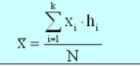
Kumulierte Häufigkeit:
Gibt an, bei welcher Anzahl der Merkmalsträger in einer empirischen Untersuchung die Merkmalsausprägung kleiner ist als eine bestimmte Schranke. Sie wird berechnet als Summe der Häufigkeiten der Merkmalsausprägungen von der kleinsten Ausprägung bis hin zu der jeweils betrachteten Schranke. |
|
|
Mean
|
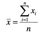
Mean (or Average Value)<br />
Most important numerical measure of location. Arithmetic average of a group of scores. The mean provides a measure of central location for the data. For a sample with n observations, the formula for the sample mean is as follows:<br /> Sum of the scores divided by the number of scores. |
|
|
Median
|
The median is the value in the middle when the data are arranged in ascending order. With an odd number of observations, the median is the middle value. An even number of observations has no middle value. In this case, we follow convention of defining the median to be the average of the two middle values.
Arrange the data in ascending order (smallest value to largest value). a) For an odd number of observations, the median is the middle value. b) For an even number of observations, the median is the average of the two middle values. |
|
|
Box-(Wisker-)Plot
|
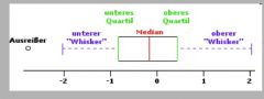
Der Box-and Wisker Plot (auch Box-Plot oder Kastengrafik) ist ein Diagramm, das zur graphischen Darstellung der Verteilung statistischer Daten verwendet wird. Er fasst dabei verschiedene robuste Streuungs- und Lagemaße in einer Darstellung zusammen.<br />
Ein Boxplot soll schnell einen Eindruck darüber vermitteln, sowohl in welchem Bereich die Daten liegen, als auch wie sich die Daten über diesen Bereich verteilen. Deshalb werden alle Werte der sogenannten Fünf-Punkte-Zusammenfassung, also der Median, die zwei Quartile und die beiden Extremwerte, dargestellt. |
|
|
Mode
|
The mode is the value that occurs with greatest frequency.
|
|
|
Graphics: Inclinations
|
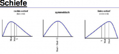
Right inclination: X (mod) < X 0,5 (median) < X (mean)
Symmetric: X (mod) = X 0,5 (median) = X (mean) Left inclination: X (mod) > X 0,5 (median) > X (mean) |
|
|
Variability
|
reflects how scores differ form one another. Variability (also called spread or dispersion) can be thought of as a measure of how different scores are from another.
Instead of comparing each score to every other score in a distribution, the one score that can be used as a comparison is the mean. |
|
|
Variance
|

The variance is a measure of variability that is based on the difference between the value of each observation (xi) and the mean. The difference between each xi and the mean is called a “deviation about the mean”.<br />
The units that are associated with the variance often cause confusion because the values being summed in the variance calculation are squared, the units associated with the variance are also squared. This squared units make it difficult to obtain an intuitive understanding and interpretation of the numerical value of the variance.<br /> Think of the variance as a measure useful in comparing the amount of variability for two or more variables. In a comparison the one with the larger variance has the most variability. Further interpretation of the value of the variance may not be necessary. |
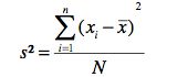
- important for the statistical distribution
- it can´t be easily compared - It can´t be interpreted from content because the dimensions are squared |
|
Standard Deviation
|
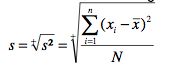
The standard deviation is defined as the positive square root of the variance. Thus, it is measured in the same units as the original data.
|
- has the same dimensions as the samples
- it can be compared because is related to the mean |
|
Coefficient of Variation
|

In some cases we are interested in a descriptive statistic that indicates how large the standard deviation is in relation to the mean. In probability theory and statistics, the coefficient of variation (CV) is a normalized measure of dispersion of a probability distribution. It is also known as unitized risk or the variation coefficient. It is defined as the ratio of the standard deviation to the mean:
|
It does not have dimensions and that is why it can be well compared.
|
|
Chi-square:
|
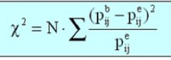
A nonparametric test that allows you to determine of what you observe in a dristrubution of frequencies would be what you would expect to occure by chance.<br />
Chi-square is the sum, over all the categories, of the squared difference between observed and expected frequencies divided by the expected frequency, multiplied by the total number of scores.<br /> p > .05 = nicht signifikant |
|
|
Cramers relationship (V)
|
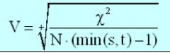
If V is higher then the statistical relationship is higher. <br />
The number is between 0 and 1. Cramer's V is a way of calculating correlation in tables which have more than 2x2 rows and columns. It is used as post-test to determine strengths of association after chi-square has determined significance. <br /> <br /> V is calculated by first calculating chi-square<br /> Chi-square says that there is a significant relationship between variables, but it does not say just how significant and important this is. Cramer's V is a post-test to give this additional information.<br /> <br /> Cramer's V varies between 0 and 1. Close to 0 it shows little association between variables. Close to 1, it indicates a strong association. |
|
|
Kind of diagram of distribution (scatter diagram) covariance
|
In the same direction: X grows and Y grows in the same tendency. Covariance is positive
No direction: No logic. Covariance is near to 0. In the opposite direction: while Y decreases X grows. Covariance is negative. |
|
|
What is Covariance
|
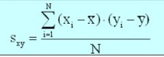
In probability theory and statistics, covariance is a measure of how much two random variables change together. If the greater values of one variable mainly correspond with the greater values of the other variable, and the same holds for the smaller values, i.e., the variables tend to show similar behavior, the covariance is positive.[1] In the opposite case, when the greater values of one variable mainly correspond to the smaller values of the other, i.e., the variables tend to show opposite behavior, the covariance is negative. The sign of the covariance therefore shows the tendency in the linear relationship between the variables. The magnitude of the covariance is not easy to interpret. The normalized version of the covariance, the correlation coefficient, however, shows by its magnitude the strength of the linear relation.
|
|
|
what is the Correlation Coefficients
|
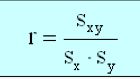
Correlation coefficients are used to measure the strength, and nature, of the relationship between two variables.<br />
Pearson‘s correlation (r), is used to calculate the correlation between two continuous (interval) variables.<br /> When you have a direct correlation, both variables change in the same direction. With an indirect correlation, variables change in opposite directions.<br /> The absolute value of the correlation coefficient reflects the strength of the correlation. Coefficients can range from -1 to +1, and the closer the absolute value is to 1, the stronger the relationship. |
|
|
Coefficient of Determination (not for exam)
|
The coefficient of determination r2 is used in the context of statistical models whose main purpose is the prediction of future outcomes on the basis of other related information. It is the proportion of variability in a data set that is accounted for by the statistical model.
It provides a measure of how well future outcomes are likely to be predicted by the model. There are several different definitions of r2 which are only sometimes equivalent. In our case, r2 is simply the square of the sample correlation coefficient. In such cases, the coefficient of determination ranges from 0 to 1. r2 is a statistic that will give some information about the goodness of fit of a model. In regression, the r2 coefficient of determination is a statistical measure of how well the regression line approximates the real data points. An r2 of 1.0 indicates that the regression line perfectly fits the data. |
|
|
Normal Probability Distribution
|
The most important probability distribution for describing a continuous random variable is the normal probability distribution. The probability density function defines the bell- shaped curve the normal probability distribution.
|
|
|
Characteristics of the Normal Probability Distribution
|
1.The entire family of normal probability distributions is differentiated by its mean and its
standard deviation. 2.The highest point of the normal curve is the mean, which is also the median and mode of the distribution. 3.The mean of the distribution can be any numerical value. |
4.The normal probability distribution is symmetric, with the shape of the curve to the left of
the mean a mirror image of the shape of the curve to the right of the mean. The tails of the curve extend to infinity in both directions and theoretically never touch the horizon. 5. The standard deviation determines how flat and wide the curve is. Larger values of the standard deviation result in wider, flatter curves, showing more variability in the data. 6.Probabilities for the normal random variable are given by areas under the curve. The total area under the curve for the normal probability distribution is 1 (this is true for all continuous probability functions). Because the distribution is symmetric, the area under the curve to the left of the mean is .50 and the area under the curve to the right of the mean is .50. |
|
Standard Normal Distribution
|
A random variable that has a normal distribution with a mean of zero and a standard deviation of one is said to have a standard normal probability distribution. The letter z [im Quatember-Buch: u] is commonly used to designate this particular normal random variable. It has the same appearance as other normal distributions, but with the special properties of μ=0 und б=1.
Probability calculations are made by computing areas under the graph of the probability density function. Thus, to find the probability that a normal random variable is within any specific interval, we must compute the area under the normal curve over that interval. For the standard normal probability distribution, areas under the normal curve have been computed and are available in tables that can be used in computing probabilities. |
|
|
Central Limit Theorem
|
The figure shows how the central limit theorem works for three different populations; each column refers to one of the populations. The top panel of the figure shows that none of the populations are normal distributed. However, note what begins to happen to the sampling distribution of the mean as the sample size is increased. When the samples are of size 2, we see that the sampling distribution of the mean begins to take on an appearance different from that of the population distribution. For samples of size 5, we see all three sampling distributions beginning to take on a bell-shaped appearance. Finally, the sample size of 30 show all three sampling distributions to be approximately normal. Thus, for sufficiently large samples, the sampling distribution of the mean can be approximated by a normal probability distribution. General statistical practice is to assume that for most applications, the sampling distribution of the mean can be approximated by a normal probability distribution
|
When the population distribution is unkown, we rely on one of the most important theorems in statistics – the central limit theorem.
In selecting simple random samples of the size n from a population, the sampling distribution of the sample mean can be approximated by a normal distribution as the sample size becomes large. The sampling distribution of the mean can be approximated by a normal probability distribution whenever the sample size is large. The large-sample condition can be assumed for the simple random samples of size 30 or more. |
|
Confidence Intervals:
|
Most statistics are used to estimate some characteristic about a population of interest, such as average household income.
Such characteristics of population are called parameters. Typically, people want to estimate the value of a parameter by taking a sample from the population and using statistics from the sample that will give them a good estimate. You take your sample result and add and subtract some number to indicate that you are giving a range of possible values for the population parameter. This number that is added to and subtracted from a statistic is called the margin of error (MOE). A statistic plus or minus a margin of error is called a confidence interval. For example, the percentage of kids who like baseball is 40 %, plus or minus 3,5 % (somewhere between 36,5 % and 43,5 %). |
The width of a confidence interval is the distance from the lower end of the interval to the upper end of the interval.
The ultimate goal when making an estimate using a confidence interval is to have a narrow width. Having to add and subtract a large margin of error only makes your result much less accurate. The relationship between margin of error and sample size: As the sample size increases, the margin of error decreases, and the confidence interval gets narrower. |
|
What is and hoe do you propose a Nullhypothesis
|
Null hypothesis:
A statement of equality between sets of variables. H0: μX = μY Research hypothesis (alternative hypothesis): A statement that there is a relationship between variables. H1: μX ǂμY H1: μX >μY |
|
|
How do you show in a table the alpha and beta error
|

|
|
|
What are the answer possibilities to the hypothesis?
|

|
|
|
Error types and correct judgement
|
Two error types: Type I error occurs when you reflect the null hypothesis when there is
actually no difference between groups or relationships between variables. Type II error occurs when you accept a false null hypothesis. This means that you conclude that there is no difference between groups or no relationship between variables when in fact there actually is. Correct judgment: First, you can accept the null hypothesis when the null hypothesis is actually true. This means that you said that there is no difference between groups, or no relationship between variables, and are correct. Secondly, you can reflect the null hypothesis when the null hypothesis is actually false. This means that you said that there is a real difference between groups, or relationship between variables, and you are correct. |
|
|
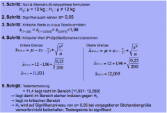
Explain the five steps of proving a hypothesis
|
|
|
|
What are the probability calculations?
|
Is to quantify the possibility that something happen according to the probability of occurrence of something.
To assign a certain event numbers that provide information about whether the arrival of these events is extremely or very likely. |
|
|
How is the distribution of percentages of the standard normal distribution?
|
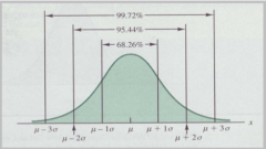
In the interval (u-o; u o) is founded two thirds of the area (68,44%). In the interval (u-o; u 2o) is foundedn 95, 44% of the area.
|
|
|
How do you calculate a relationship between different types of variables?
|
Metric and ordinal: like 2 ordinal variables.
Metric and nominal: like 2 nominal variables Ordinal and nominal: like 2 nominal variables. |
|
|
Rules for the graphic representation
|
- names of x and y axis
- zero of the percentage value must be on the y axis in the intersection with x axis - avoid 3D graphs - maintain order of the variables - use direct name before legends |